Basis for subplot2grid, ticker, enumerate, seaborn, plt/ax/fig
Some things I discovered while reading other people’s code that I hadn’t mastered yet.
matplotlib.ticker
Locating
Tick locating
The Locator class is the base class for all tick locators. The locators handle autoscaling of the view limits based on the data limits, and the choosing of tick locations. A useful semi-automatic tick locator is MultipleLocator. It is initialized with a base, e.g., 10, and it picks axis limits and ticks that are multiples of that base.
The Locator subclasses defined here are
MaxNLocatorwith simple defaults. This is the default tick locator for most plotting.Finds up to a max number of intervals with ticks at nice locations.
Space ticks evenly from min to max.
Space ticks logarithmically from min to max.
Ticks and range are a multiple of base; either integer or float.
Tick locations are fixed.
Locator for index plots (e.g., where
x = range(len(y))).No ticks.
Locator for use with with the symlog norm; works like
LogLocatorfor the part outside of the threshold and adds 0 if inside the limits.Locator for logit scaling.
Choose a
MultipleLocatorand dynamically reassign it for intelligent ticking during navigation.Locator for minor ticks when the axis is linear and the major ticks are uniformly spaced. Subdivides the major tick interval into a specified number of minor intervals, defaulting to 4 or 5 depending on the major interval.
There are a number of locators specialized for date locations - see the dates module.
You can define your own locator by deriving from Locator. You must override the __call__ method, which returns a sequence of locations, and you will probably want to override the autoscale method to set the view limits from the data limits.
If you want to override the default locator, use one of the above or a custom locator and pass it to the x or y axis instance. The relevant methods are:
ax.xaxis.set_major_locator(xmajor_locator)
ax.xaxis.set_minor_locator(xminor_locator)
ax.yaxis.set_major_locator(ymajor_locator)
ax.yaxis.set_minor_locator(yminor_locator)
The default minor locator is NullLocator, i.e., no minor ticks on by default.
Formatting
Tick formatting
Tick formatting is controlled by classes derived from Formatter. The formatter operates on a single tick value and returns a string to the axis.
No labels on the ticks.
Set the strings from a list of labels.
Set the strings manually for the labels.
User defined function sets the labels.
Use string
formatmethod.Use an old-style sprintf format string.
Default formatter for scalars: autopick the format string.
Formatter for log axes.
Format values for log axis using
exponent = log_base(value).Format values for log axis using
exponent = log_base(value)using Math text.Format values for log axis using scientific notation.
Probability formatter.
Format labels in engineering notation
Format labels as a percentage
You can derive your own formatter from the Formatter base class by simply overriding the __call__ method. The formatter class has access to the axis view and data limits.
To control the major and minor tick label formats, use one of the following methods:
ax.xaxis.set_major_formatter(xmajor_formatter)
ax.xaxis.set_minor_formatter(xminor_formatter)
ax.yaxis.set_major_formatter(ymajor_formatter)
ax.yaxis.set_minor_formatter(yminor_formatter)
See Major and minor ticks for an example of setting major and minor ticks. See the matplotlib.dates module for more information and examples of using date locators and formatters.
Reference
https://matplotlib.org/3.1.1/api/ticker_api.html
enumerate
Description
The enumerate() function is used to combine an iterable data object (such as a list, tuple, or string) into an index sequence, listing both the data and its index, generally used in for loops.
Available in Python 2.3 and above, start parameter added in 2.6.
Syntax
The syntax for the enumerate() method is:
enumerate(sequence, [start=0])Parameters
- sequence — A sequence, iterator, or other object that supports iteration.
- start — Starting position of the index.
Return Value
Returns an enumerate object.
Examples
The following shows examples of using the enumerate() method:
>>>seasons = ['Spring', 'Summer', 'Fall', 'Winter']
>>> list(enumerate(seasons))
[(0, 'Spring'), (1, 'Summer'), (2, 'Fall'), (3, 'Winter')]
>>> list(enumerate(seasons, start=1))       # index starts from 1
[(1, 'Spring'), (2, 'Summer'), (3, 'Fall'), (4, 'Winter')]
Regular for loop
>>>i = 0
>>> seq = ['one', 'two', 'three']
>>> for element in seq:
...     print i, seq[i]
...     i +=1
...
0 one
1 two
2 three
for loop using enumerate
>>>seq = ['one', 'two', 'three']
>>> for i, element in enumerate(seq):
...     print i, element
...
0 one
1 two
2 three
Reference
https://www.runoob.com/python/python-func-enumerate.html
subplot2grid
This allows you to customize the position of subplots and span across original sizes.
Original: https://wizardforcel.gitbooks.io/matplotlib-user-guide/content/3.3.html
GridSpecSpecifies the geometry of the grid where the subplot will be placed. You need to set the number of rows and columns of the grid. Subplot layout parameters (e.g., left, right, etc.) can be optionally adjusted.
SubplotSpecSpecifies the subplot position in a given GridSpec.
subplot2gridA helper function similar to pyplot.subplot, but uses 0-based indexing and allows subplots to span multiple cells.
subplot2grid Basic Example
To use subplot2grid, you need to provide the geometry of the grid and the position of the subplot in the grid. For a simple single-cell subplot:
ax = plt.subplot2grid((2,2),(0, 0))Equivalent to:
ax = plt.subplot(2,2,1)
       nRow=2, nCol=2
(0,0) +-------+-------+
      |   1   |       |
      +-------+-------+
      |       |       |
      +-------+-------+
Note that unlike subplot, indices in gridspec start from 0.
To create subplots that span multiple cells,
ax2 = plt.subplot2grid((3,3), (1, 0), colspan=2)
ax3 = plt.subplot2grid((3,3), (1, 2), rowspan=2)
For example, the following commands:
ax1 = plt.subplot2grid((3,3), (0,0), colspan=3)
ax2 = plt.subplot2grid((3,3), (1,0), colspan=2)
ax3 = plt.subplot2grid((3,3), (1, 2), rowspan=2)
ax4 = plt.subplot2grid((3,3), (2, 0))
ax5 = plt.subplot2grid((3,3), (2, 1))
Will create:

GridSpec and SubplotSpec
You can explicitly create GridSpec and use them to create subplots.
For example,
ax = plt.subplot2grid((2,2),(0, 0))Equivalent to:
import matplotlib.gridspec as gridspec
gs = gridspec.GridSpec(2, 2)
ax = plt.subplot(gs[0, 0])
The gridspec example provides array-like (1D or 2D) indexing and returns SubplotSpec instances. For example, using slicing to return SubplotSpec instances that span multiple cells.
The above example becomes:
gs = gridspec.GridSpec(3, 3)
ax1 = plt.subplot(gs[0, :])
ax2 = plt.subplot(gs[1,:-1])
ax3 = plt.subplot(gs[1:, -1])
ax4 = plt.subplot(gs[-1,0])
ax5 = plt.subplot(gs[-1,-2])
Adjusting GridSpec Layout
When explicitly using GridSpec, you can adjust the layout parameters of subplots created by gridspec.
gs1 = gridspec.GridSpec(3, 3)
gs1.update(left=0.05, right=0.48, wspace=0.05)
This is similar to subplots_adjust, but it only affects subplots created from the given GridSpec.
The following code
gs1 = gridspec.GridSpec(3, 3)
gs1.update(left=0.05, right=0.48, wspace=0.05)
ax1 = plt.subplot(gs1[:-1, :])
ax2 = plt.subplot(gs1[-1, :-1])
ax3 = plt.subplot(gs1[-1, -1])

gs2 = gridspec.GridSpec(3, 3)
gs2.update(left=0.55, right=0.98, hspace=0.05)
ax4 = plt.subplot(gs2[:, :-1])
ax5 = plt.subplot(gs2[:-1, -1])
ax6 = plt.subplot(gs2[-1, -1])
Will produce

Creating GridSpec from SubplotSpec
You can create GridSpec from SubplotSpec, where its layout parameters are set to the layout parameters of the given SubplotSpec position.
gs0 = gridspec.GridSpec(1, 2)

gs00 = gridspec.GridSpecFromSubplotSpec(3, 3, subplot_spec=gs0[0])
gs01 = gridspec.GridSpecFromSubplotSpec(3, 3, subplot_spec=gs0[1])
Creating Complex Nested GridSpec with SubplotSpec
Here’s a more complex example of nested gridspec, where we place a box around each cell of a 4x4 outer grid by hiding appropriate spines in each 3x3 inner grid.

GridSpec with Variable Grid Sizes
Normally, GridSpec creates grids of equal size. You can adjust the relative heights and widths of rows and columns. Note that absolute height values are meaningless; only their relative ratios matter.
gs = gridspec.GridSpec(2, 2,
                       width_ratios=[1,2],
                       height_ratios=[4,1]
                       )

ax1 = plt.subplot(gs[0])
ax2 = plt.subplot(gs[1])
ax3 = plt.subplot(gs[2])
ax4 = plt.subplot(gs[3])
seaborn
seaborn is a further encapsulation of matplotlib, simply put, it’s easier to use.
Official website: https://seaborn.pydata.org/
Here are some code snippets I think will be useful.
lineplot
seaborn.lineplot(x=None, y=None, hue=None, size=None, style=None, data=None, palette=None, hue_order=None, hue_norm=None, sizes=None, size_order=None, size_norm=None, dashes=True, markers=None, style_order=None, units=None, estimator=‘mean’, ci=95, n_boot=1000, seed=None, sort=True, err_style=‘band’, err_kws=None, legend=‘brief’, ax=None, **kwargs)
https://seaborn.pydata.org/generated/seaborn.lineplot.html
heatmap
seaborn.heatmap(data, vmin=None, vmax=None, cmap=None, center=None, robust=False, annot=None, fmt=’.2g’, annot_kws=None, linewidths=0, linecolor=‘white’, cbar=True, cbar_kws=None, cbar_ax=None, square=False, xticklabels=‘auto’, yticklabels=‘auto’, mask=None, ax=None, **kwargs)
https://zhuanlan.zhihu.com/p/35494575
lmplot
seaborn.lmplot(x, y, data, hue=None, col=None, row=None, palette=None, col_wrap=None, size=5, aspect=1, markers=‘o’, sharex=True, sharey=True, hue_order=None, col_order=None, row_order=None, legend=True, legend_out=True, x_estimator=None, x_bins=None, x_ci=‘ci’, scatter=True, fit_reg=True, ci=95, n_boot=1000, units=None, order=1, logistic=False, lowess=False, robust=False, logx=False, x_partial=None, y_partial=None, truncate=False, x_jitter=None, y_jitter=None, scatter_kws=None, line_kws=None)
https://zhuanlan.zhihu.com/p/25909753
Common statistical plots can basically be found here
https://seaborn.pydata.org/examples/index.html
subplot_adjust
matplotlib.pyplot.subplots_adjust(*args, **kwargs)
subplots_adjust(left=None, bottom=None, right=None, top=None,wspace=None, hspace=None)

left  = 0.125  # distance from subplot to figure left edge
right = 0.9    # right edge
bottom = 0.1   # bottom
top = 0.9      # top
wspace = 0.2   # horizontal spacing between subplots
hspace = 0.2   # vertical spacing between subplots
plt/ax/fig
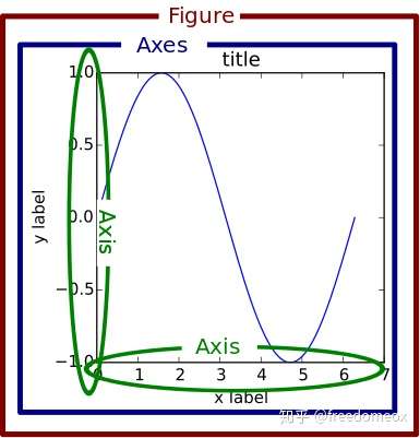
Try to avoid using plt directly