Python描画基礎
この2日間、描画の整理をしていて、matplotlibの知識が本当に不足していることに気づきました。このノートはcartopy以外で使うものを整理するためのものです。
matplotlib
基礎知識
Matplotlibで最も重要な基礎概念はfigureとaxesです。
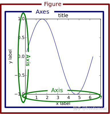
Matplotlibでは、figureは描画ボード、axesはキャンバス、axisは座標軸を意味します。例えば:
x = np.linspace(0, 10, 20)  # データ生成
y = x * x + 2

fig = plt.figure()  # 新しいfigureオブジェクトを作成
axes = fig.add_axes([0.5, 0.5, 0.8, 0.8])  # キャンバスの左、下、幅、高さを制御
axes.plot(x, y, 'r')
同じ描画ボード上に複数のキャンバスを描くことができます:
fig = plt.figure()  # 新しい描画ボードを作成
axes1 = fig.add_axes([0.1, 0.1, 0.8, 0.8])  # 大きいキャンバス
axes2 = fig.add_axes([0.2, 0.5, 0.4, 0.3])  # 小さいキャンバス

axes1.plot(x, y, 'r')  # 大きいキャンバス
axes2.plot(y, x, 'g')  # 小さいキャンバス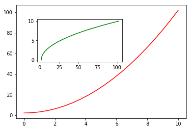
また、plt.subplots()を使ってキャンバスを追加する方法もあります:
fig, axes = plt.subplots(nrows=1, ncols=2)  # サブプロット:1行、2列
for ax in axes:
    ax.plot(x, y, 'r')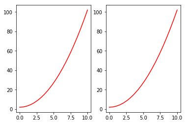
1つのキャンバスだけを描く場合でも、plt.plot()ではなくfig, axes = plt.subplots()を使用することをお勧めします。
基本スタイル調整
タイトルと凡例の追加
タイトル、軸ラベル、凡例を含む図形を描画:
fig, axes = plt.subplots()

axes.set_xlabel('x label')  # X軸ラベル
axes.set_ylabel('y label')
axes.set_title('title')  # 図のタイトル

axes.plot(x, x**2)
axes.plot(x, x**3)
axes.legend(["y = x**2", "y = x**3"], loc=0)  # 凡例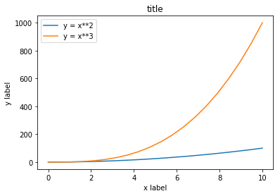
凡例のlocパラメータは凡例の位置を示します。1, 2, 3, 4はそれぞれ右上、左上、左下、右下を表し、0は自動適応を意味します。
線のスタイル、色、透明度
fig, axes = plt.subplots()

axes.plot(x, x+1, color="red", alpha=0.5)
axes.plot(x, x+2, color="#1155dd")
axes.plot(x, x+3, color="#15cc55")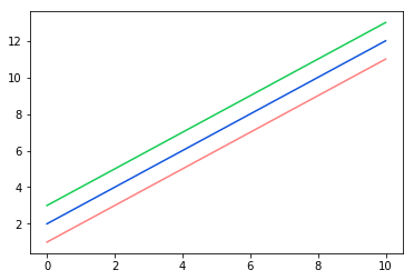
グリッドと軸範囲
fig, axes = plt.subplots(1, 2, figsize=(10, 5))

# グリッドを表示
axes[0].plot(x, x**2, x, x**3, lw=2)
axes[0].grid(True)

# 軸範囲を設定
axes[1].plot(x, x**2, x, x**3)
axes[1].set_ylim([0, 60])
axes[1].set_xlim([2, 5])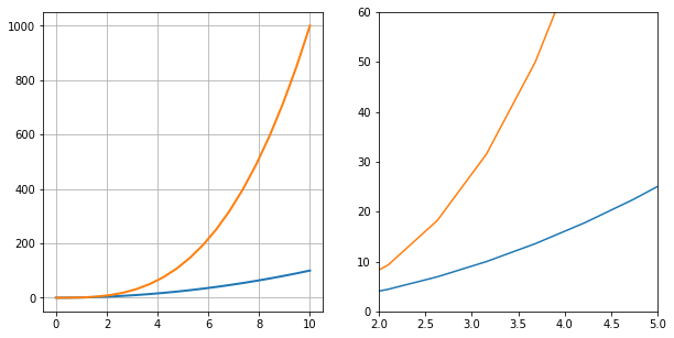
チートシート
Matplotlib公式がチートシートを提供しています:
https://github.com/matplotlib/cheatsheets
3Dグラフィックス
Matplotlibは3Dグラフィックスも描画できます。3Dグラフィックスは主にmplot3dモジュールで実装されます。
import numpy as np
from mpl_toolkits.mplot3d import Axes3D
import matplotlib.pyplot as plt

x = np.random.normal(0, 1, 100)
y = np.random.normal(0, 1, 100)
z = np.random.normal(0, 1, 100)

fig = plt.figure()
ax = Axes3D(fig)
ax.scatter(x, y, z)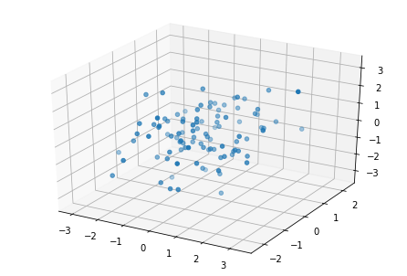
3D曲面プロット:
fig = plt.figure()
ax = Axes3D(fig)

X = np.arange(-2, 2, 0.1)
Y = np.arange(-2, 2, 0.1)
X, Y = np.meshgrid(X, Y)
Z = np.sqrt(X ** 2 + Y ** 2)

ax.plot_surface(X, Y, Z, cmap=plt.cm.winter)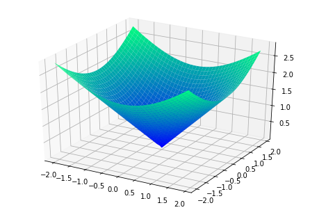
seaborn
SeabornはMatplotlibコアライブラリの上に構築された高レベルAPIで、より美しいグラフィックスを簡単に描画できます。
クイック最適化
import seaborn as sns

sns.set()  # Seabornスタイルを宣言

plt.bar(x, y_bar)
plt.plot(x, y_line, '-o', color='y')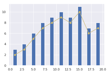
関連プロット
iris = sns.load_dataset("iris")
sns.relplot(x="sepal_length", y="sepal_width", hue="species", data=iris)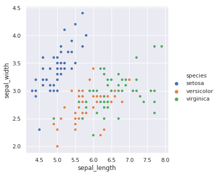
カテゴリプロット
カテゴリプロットのFigureレベルインターフェースはcatplotです。以下が含まれます:
- カテゴリ散布図:
stripplot()、swarmplot() - カテゴリ分布:
boxplot()、violinplot()、boxenplot() - カテゴリ推定:
pointplot()、barplot()、countplot()
sns.catplot(x="sepal_length", y="species", data=iris)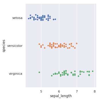
箱ひげ図:
sns.catplot(x="sepal_length", y="species", kind="box", data=iris)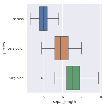
バイオリンプロット:
sns.catplot(x="sepal_length", y="species", kind="violin", data=iris)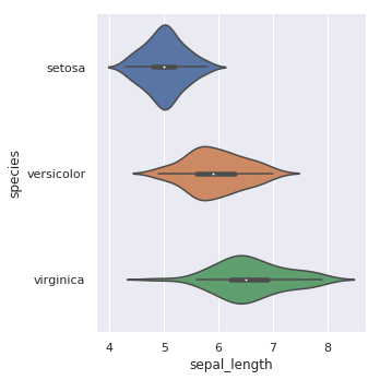
分布プロット
分布プロットは変数の分布を可視化するために使用されます。Seabornはjointplot、pairplot、distplot、kdeplotを提供しています。
sns.distplot(iris["sepal_length"])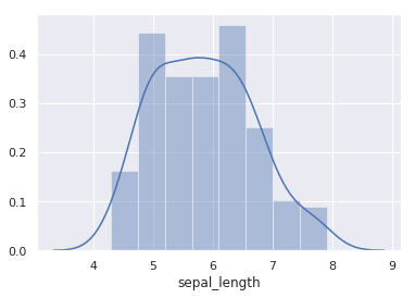
jointplotは二変量分布に使用されます:
sns.jointplot(x="sepal_length", y="sepal_width", data=iris)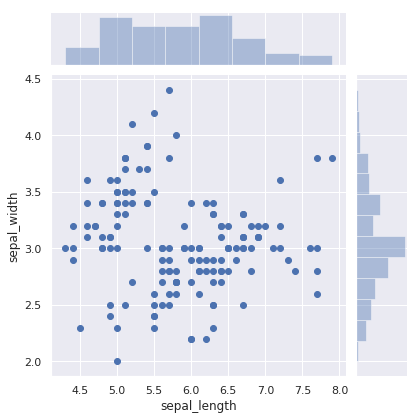
pairplotはすべての特徴量のペアワイズ比較をサポートします:
sns.pairplot(iris, hue="species")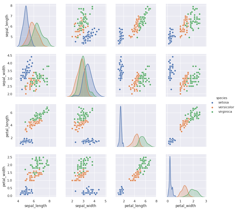
回帰プロット
回帰プロット関数:lmplotとregplot。
sns.regplot(x="sepal_length", y="sepal_width", data=iris)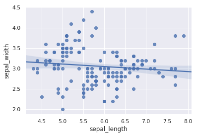
lmplotは比較のために第三次元を導入することをサポートします:
sns.lmplot(x="sepal_length", y="sepal_width", hue="species", data=iris)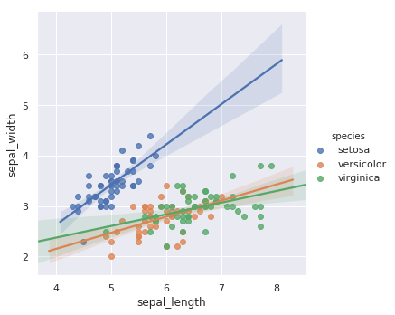
マトリックスプロット
最もよく使われるのはheatmapとclustermapです。
import numpy as np

sns.heatmap(np.random.rand(10, 10))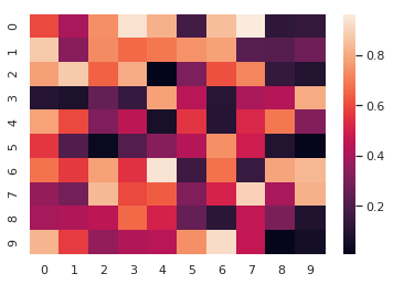
ヒートマップは特定のシナリオで非常に便利です。例えば、変数の相関係数ヒートマップを描画する場合などです。