Scipy optimize
主要是几个常用的
minimize
Least_square
nnls
Lsq_linear
Curve_fit
另外附带一个numpy.linalg.lstsq
另外我发现了一个非常及乖的东西,一般都得x作为func的第一个参数才能拟合好
minimize
这个主要是用来代替matlab中的fminunc
scipy.optimize.minimize(fun, x0, args=(), method=None, jac=None, hess=None, hessp=None, bounds=None, constraints=(), tol=None, callback=None, options=None)fun就是要去最小化的cost func,对cost func的要求是
fun
The objective function to be minimized.
fun(x, *args) -> float
where x is an 1-D array with shape (n,) and args is a tuple of the fixed parameters needed to completely specify the function.
x0是初始化的参数,也就是常说的initial guess. Array of real elements of size (n,), where ‘n’ is the number of independent variables.
method:该参数代表采用的方式,默认是BFGS, L-BFGS-B, SLSQP中的一种,可选TNC,
jac是用来计算梯度的方法,这个大多数时候可以忽略,也就是雅各比矩阵
options:用来控制最大的迭代次数,以字典的形式来进行设置,例如:options={‘maxiter’
}boundssequence or
Bounds, optionalBounds on variables for L-BFGS-B, TNC, SLSQP, Powell, and trust-constr methods. There are two ways to specify the bounds:
- Instance of
Boundsclass.- Sequence of
(min, max)pairs for each element in x. None is used to specify no bound.constraints{Constraint, dict} or List of {Constraint, dict}, optional
Constraints definition (only for COBYLA, SLSQP and trust-constr).
Constraints for ‘trust-constr’ are defined as a single object or a list of objects specifying constraints to the optimization problem. Available constraints are:
bounds主要是用来控制上下界,constraions则是通过变量间的关系来缩小范围
tol: float, optional
Tolerance for termination. For detailed control, use solver-specific options.
Tol 是最小迭代值,就是迭代停止的条件
Here is the example of Rosenbrock function
import numpy as np
from scipy.optimize import minimize
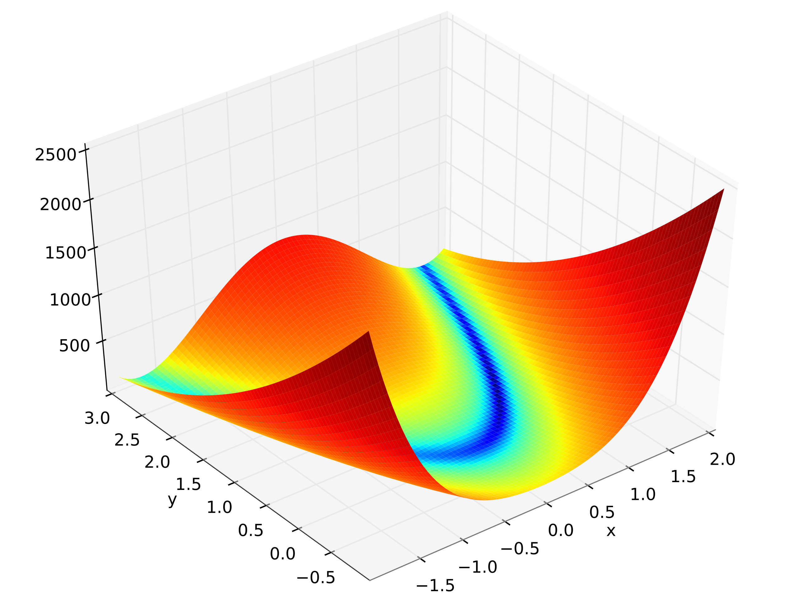
def rosen(x):
"""The Rosenbrock function"""
return sum(100.0*(x[1:]-x[:-1]**2.0)**2.0 + (1-x[:-1])**2.0)
x0 = np.array([1.3, 0.7, 0.8, 1.9, 1.2])
res = minimize(rosen, x0, method='nelder-mead',
options={'xatol': 1e-8, 'disp': True})
Optimization terminated successfully.
Current function value: 0.000000
Iterations: 339
Function evaluations: 571
>>>
print(res.x)
[1. 1. 1. 1. 1.]More often, we need to use the boudnarrays or constrains. Here I show the boundary
Least_square
scipy.optimize.least_squares(fun, x0, jac='2-point', bounds=- inf, inf, method='trf', ftol=1e-08, xtol=1e-08, gtol=1e-08, x_scale=1.0, loss='linear', f_scale=1.0, diff_step=None, tr_solver=None, tr_options={}, jac_sparsity=None, max_nfev=None, verbose=0, args=(), kwargs={})这个与上一个几乎一样
nnls
scipy.optimize.nnls(A, b, maxiter=None)Solve argmin_x || Ax - b ||_2 for x>=0.
Parameters
**A **ndarray
Matrix
Aas shown above.**b ** ndarray
Right-hand side vector.
maxiter: int, optional
Maximum number of iterations, optional. Default is
3 * A.shape[1].
Returns
**x ** ndarray
Solution vector.
**rnorm: float
The residual,
|| Ax-b ||_2.
lsq_linear
scipy.optimize.lsq_linear(A, b, bounds=- inf, inf, method='trf', tol=1e-10, lsq_solver=None, lsmr_tol=None, max_iter=None, verbose=0)Solve a linear least-squares problem with bounds on the variables.
Given a m-by-n design matrix A and a target vector b with m elements, lsq_linear solves the following optimization problem:
minimize 0.5 * ||A x - b||**2
subject to lb <= x <= ub
curve_fit
scipy.optimize.curve_fit(f, xdata, ydata, p0=None, sigma=None, absolute_sigma=False, check_finite=True, bounds=- inf, inf, method=None, jac=None, **kwargs)这个其实是最常用的一个函数
需要注意 这里的f并不是cost func,而是model func,例如
def f_1(x, A, B):
return A * x + B- **xdata array_like or object **The independent variable where the data is measured. Should usually be an M-length sequence or an (k,M)-shaped array for functions with k predictors, but can actually be any object.[1] 简单说就是要拟合的自变量数组
- **ydata array_like **The dependent data, a length M array - nominally
f(xdata,...).[1] 简单说就是要拟合的因变量的值 - p0 array_like , optionalInitial guess for the parameters (length N). If None, then the initial values will all be 1 (if the number of parameters for the function can be determined using introspection, otherwise a ValueError is raised).[1] 就是给你的函数的参数确定一个初始值来减少计算机的计算量
- Method to use for optimization. See
least_squaresfor more details. Default is ‘lm’ for unconstrained problems and ‘trf’ if bounds are provided. The method ‘lm’ won’t work when the number of observations is less than the number of variables, use ‘trf’ or ‘dogbox’ in this case.
这里放一下官方例子
import matplotlib.pyplot as plt
from scipy.optimize import curve_fit
def func(x, a, b, c):
return a * np.exp(-b * x) + cDefine the data to be fit with some noise:
xdata = np.linspace(0, 4, 50)
y = func(xdata, 2.5, 1.3, 0.5)
np.random.seed(1729)
y_noise = 0.2 * np.random.normal(size=xdata.size)
ydata = y + y_noise
plt.plot(xdata, ydata, 'b-', label='data'
it for the parameters a, b, c of the function func:
popt, pcov = curve_fit(func, xdata, ydata)
popt

plt.plot(xdata, func(xdata, *popt), 'r-',
         label='fit: a=%5.3f, b=%5.3f, c=%5.3f' % tuple(popt))
Constrain the optimization to the region of 0 <= a <= 3, 0 <= b <= 1 and 0 <= c <= 0.5:
popt, pcov = curve_fit(func, xdata, ydata, bounds=(0, [3., 1., 0.5]))
popt

plt.plot(xdata, func(xdata, *popt), 'g--',
label='fit: a=%5.3f, b=%5.3f, c=%5.3f' % tuple(popt))plt.xlabel('x')
plt.ylabel('y')
plt.legend()
plt.show()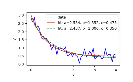
但是这里有个问题,如果我想固定a的值,或者我想得到一串的函数每个函数都有固定的a的值,该怎么办呢?
这种时候其实就需要把a不视为变量,再次建立一个函数 把a传进去,例如
custom_gaussian = lambda x, mu: gaussian(x, mu, 0.05)利用lambda建立了小的匿名函数
import matplotlib.pyplot as plt
import numpy as np
import scipy.optimize

def gaussian(x, mu, sigma):
    return 1 / sigma / np.sqrt(2 * np.pi) * np.exp(-(x - mu)**2 / 2 / sigma**2)
# This is the original, full parameter gaussion function
# Create sample data
x = np.linspace(0, 2, 200)
y = gaussian(x, 1, 0.1) + np.random.rand(*x.shape) - 0.5
plt.plot(x, y, label="sample data")

# Fit with original fit function
popt, _ = scipy.optimize.curve_fit(gaussian, x, y)
plt.plot(x, gaussian(x, *popt), label="gaussian")

# Fit with custom fit function with fixed `sigma`
custom_gaussian = lambda x, mu: gaussian(x, mu, 0.05)
# this is the customed gaussion function that we want to fuit
popt, _ = scipy.optimize.curve_fit(custom_gaussian, x, y)
plt.plot(x, custom_gaussian(x, *popt), label="custom_gaussian")

plt.legend()
plt.show()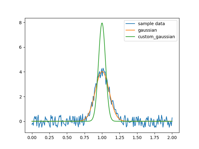
numpy.linalg.lstsq
这个是numpy自带的the least-squares solution to a linear matrix equation.
这里需要回忆一下线性方程组的问题
这个大括号的排版是不是有点问题
其中的以及等等是已知的常数,而等等则是要求的未知数。
如果用线性代数的概念来表达,线性方程组则可以写成
这里的A是m×n 矩阵,x是含有n个元素列向量,b是含有m 个元素列向量。
如果有一组数x1、x2、……xn使得方程组的等号都成立,那么这组数就叫做方程组的解。一个线性方程组的所有的解的集合会被简称为解集。根据解的存在情况,线性方程组可以分为三类:
有唯一解的恰定方程组,
解不存在的超定方程组,
有无穷多解的欠定方程组(也被通俗地称为不定方程组)。
线性代数基本就是讲了怎判断有没有解和怎么求解这两件事
想复习线性方程组可以看/Users/zhenjia/hexoblog/source/_posts/Scipy-optimize/线性方程组.pdf
不严格地说,当m>n的时候一般没有解,成为超定方程组,但是这种时候可以把问题转化为优化问题,即求一组x使得最小,这就是个最小二乘问题
Parameters
a(M, N) array_like
“Coefficient” matrix.
b{(M,), (M, K)} array_like
Ordinate or “dependent variable” values. If b is two-dimensional, the least-squares solution is calculated for each of the K columns of b.
rcondfloat, optional
Cut-off ratio for small singular values of a. For the purposes of rank determination, singular values are treated as zero if they are smaller than rcond times the largest singular value of a.Changed in version 1.14.0: If not set, a FutureWarning is given. The previous default of
-1will use the machine precision as rcond parameter, the new default will use the machine precision times max(M, N). To silence the warning and use the new default, usercond=None, to keep using the old behavior, usercond=-1.
Returns
x{(N,), (N, K)} ndarray
Least-squares solution. If b is two-dimensional, the solutions are in the K columns of x.
residuals{(1,), (K,), (0,)} ndarray
Sums of residuals; squared Euclidean 2-norm for each column in
b - a*x. If the rank of a is < N or M <= N, this is an empty array. If b is 1-dimensional, this is a (1,) shape array. Otherwise the shape is (K,).rankint
Rank of matrix a.
s(min(M, N),) ndarray
Singular values of a.
Examples fot
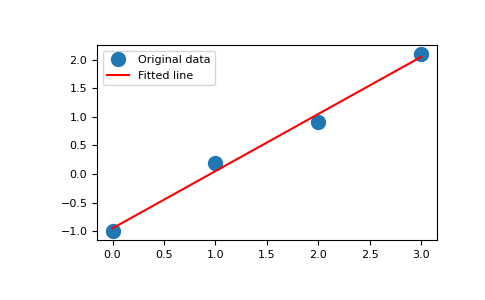
x = np.array([0, 1, 2, 3])
y = np.array([-1, 0.2, 0.9, 2.1])
By examining the coefficients, we see that the line should have a gradient of roughly 1 and cut the y-axis at, more or less, -1.
We can rewrite the line equation as y = Ap, where A = [[x 1]] and p = [[m], [c]]. Now use lstsq to solve for p:
A = np.vstack([x, np.ones(len(x))]).T
>>> A
array([[ 0.,  1.],
       [ 1.,  1.],
       [ 2.,  1.],
       [ 3.,  1.]])
m, c = np.linalg.lstsq(A, y, rcond=None)[0]
>>> m, c
(1.0 -0.95) # may varyimport matplotlib.pyplot as plt
>>> _ = plt.plot(x, y, 'o', label='Original data', markersize=10)
>>> _ = plt.plot(x, m*x + c, 'r', label='Fitted line')
>>> _ = plt.legend()
>>> plt.show()